These plots are some of the figures I used in my graduate thesis. For more information: DEMAND FOR RESIDENTIAL SOLAR PHOTOVOLTAIC SYSTEMS: EVIDENCE FROM NOVA SCOTIA
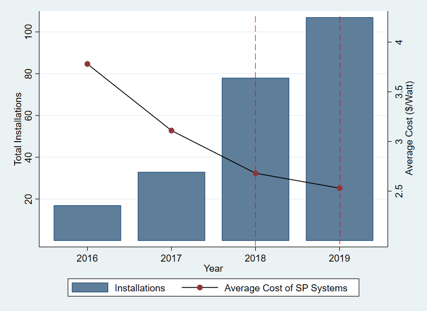
Figure 1 depicts the number of SP system installations in NS from 2016 to 2019. Rebate of $1/Watt was introduced in 2018 and the total number of installations in 2018 was 78 compared to 33 in 2017. While rebate decreased to $0.85/Watt on March 26, 2019, the total number of installations increased.

Figure 1: Number of Installations Vs Installations Cost
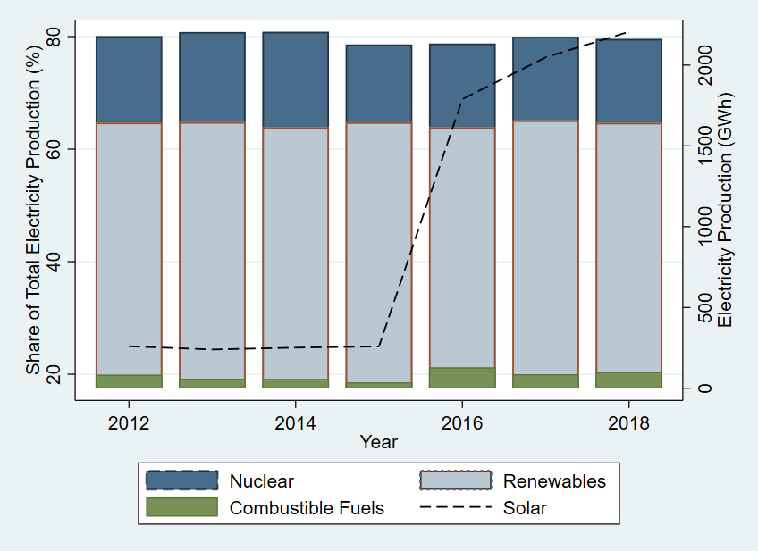
Figure 2 shows the change in percentage contribution of nuclear, renewables and combustible fuels to the total electricity production along with total electricity produced by SP systems (secondary axis) in several provinces in Canada from 2012 to 2018. Total electricity generation in 2012 and 2015 was 595 TWh and 593 TWh respectively, a 0.3% decrease. During this period both total and percentage of electricity generation using combustible fuels decreased, while total electricity production using non-GHG emitting sources increased from 463 TWh to 483 TWh, a 6% increase.

Figure 2: Number of Installations Vs Installations Cost
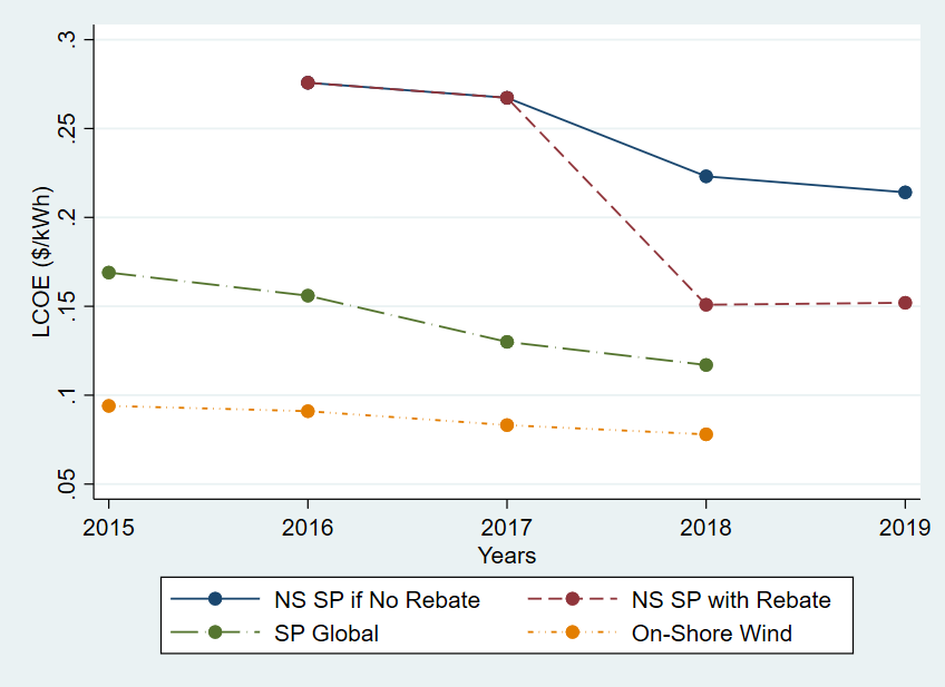
Levelized cost of electricity (LCOE), on the other hand, compares the cost of different sources of energy production. The absolute cost to produce electricity by different sources cannot be compared as the cost varies by region, project, capital cost, maintenance cost, and many other variables. LCOE takes into consideration all the different factors that affect electricity price and normalizes it to a comparable value in $/kWh.
Figure 3 shows the change in LCOE ($/kWh) of on-shore wind and SP systems in the world and NS. LCOE has been decreasing for all renewable energy sources with on-shore wind incurring the lowest cost to produce a kWh of electricity. The SP systems in NS that benefited from a $1/Watt rebate in 2018, the LCOE is 0.151 $/kWh which is a 44% decrease compared to SP systems installed in 2017.

Figure 3: Levelized Cost of Electricity for Different Renewable Sources
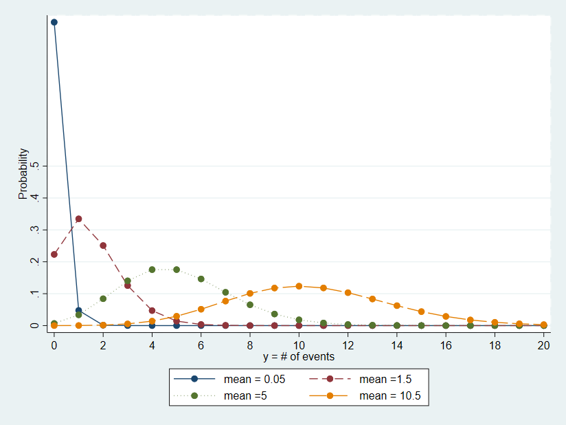
Generating Poission distribution for different mean values in STATA: Figure 4.
clear all
set obs 21
gen k = _n - 1
label var k "y = # of events"
gen psn1 = poissonp(0.05, k)
label var psn1 "mean = 0.05"
gen psn2 = poissonp(1.5, k)
label var psn2 "mean =1.5"
gen psn3 = poissonp(5, k)
label var psn3 "mean =5"
gen psn4 = poissonp(10.5, k)
label var psn4 "mean = 10.5"
graph twoway connected psn1 psn2 psn3 psn4 k, ytitle("Probability") \\
ylabel(0(.1) .5) xlabel(0(2)20)\\
lwidth(thin thin thin thin) msymbol(0 D S T)
Figure 4: Number of Installations Vs Installations Cost